14.4 0-1 Knapsack problem
The knapsack problem is an excellent introductory problem for dynamic programming and is the most common type of problem in dynamic programming. It has many variants, such as the 0-1 knapsack problem, the unbounded knapsack problem, and the multiple knapsack problem, etc.
In this section, we will first solve the most common 0-1 knapsack problem.
Question
Given \(n\) items, the weight of the \(i\)-th item is \(wgt[i-1]\) and its value is \(val[i-1]\), and a knapsack with a capacity of \(cap\). Each item can be chosen only once. What is the maximum value of items that can be placed in the knapsack under the capacity limit?
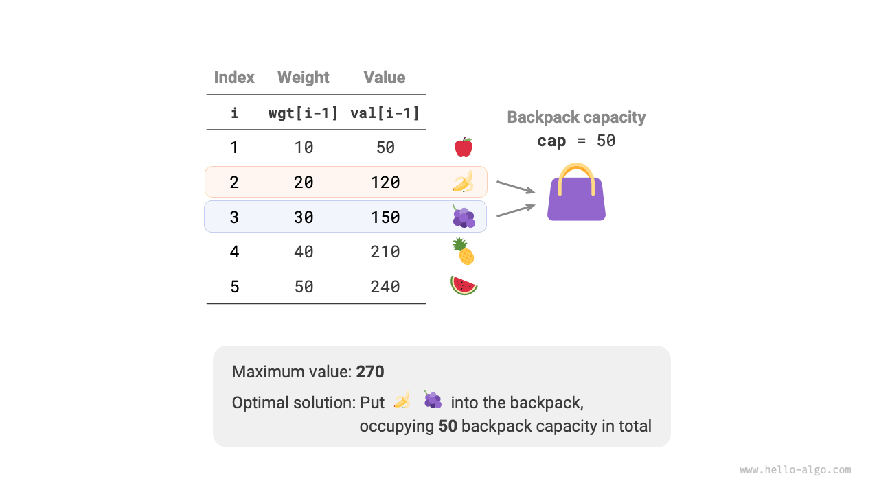
Observe Figure 14-17, since the item number \(i\) starts counting from 1, and the array index starts from 0, thus the weight of item \(i\) corresponds to \(wgt[i-1]\) and the value corresponds to \(val[i-1]\).
Figure 14-17 Example data of the 0-1 knapsack
We can consider the 0-1 knapsack problem as a process consisting of \(n\) rounds of decisions, where for each item there are two decisions: not to put it in or to put it in, thus the problem fits the decision tree model.
The objective of this problem is to "maximize the value of the items that can be put in the knapsack under the limited capacity," thus it is more likely a dynamic programming problem.
First step: Think about each round of decisions, define states, thereby obtaining the \(dp\) table
For each item, if not put into the knapsack, the capacity remains unchanged; if put in, the capacity is reduced. From this, the state definition can be obtained: the current item number \(i\) and knapsack capacity \(c\), denoted as \([i, c]\).
State \([i, c]\) corresponds to the sub-problem: the maximum value of the first \(i\) items in a knapsack of capacity \(c\), denoted as \(dp[i, c]\).
The solution we are looking for is \(dp[n, cap]\), so we need a two-dimensional \(dp\) table of size \((n+1) \times (cap+1)\).
Second step: Identify the optimal substructure, then derive the state transition equation
After making the decision for item \(i\), what remains is the sub-problem of decisions for the first \(i-1\) items, which can be divided into two cases.
- Not putting item \(i\): The knapsack capacity remains unchanged, state changes to \([i-1, c]\).
- Putting item \(i\): The knapsack capacity decreases by \(wgt[i-1]\), and the value increases by \(val[i-1]\), state changes to \([i-1, c-wgt[i-1]]\).
The above analysis reveals the optimal substructure of this problem: the maximum value \(dp[i, c]\) is equal to the larger value of the two schemes of not putting item \(i\) and putting item \(i\). From this, the state transition equation can be derived:
It is important to note that if the current item's weight \(wgt[i - 1]\) exceeds the remaining knapsack capacity \(c\), then the only option is not to put it in the knapsack.
Third step: Determine the boundary conditions and the order of state transitions
When there are no items or the knapsack capacity is \(0\), the maximum value is \(0\), i.e., the first column \(dp[i, 0]\) and the first row \(dp[0, c]\) are both equal to \(0\).
The current state \([i, c]\) transitions from the state directly above \([i-1, c]\) and the state to the upper left \([i-1, c-wgt[i-1]]\), thus, the entire \(dp\) table is traversed in order through two layers of loops.
Following the above analysis, we will next implement the solutions in the order of brute force search, memoized search, and dynamic programming.
1. Method one: Brute force search
The search code includes the following elements.
- Recursive parameters: State \([i, c]\).
- Return value: Solution to the sub-problem \(dp[i, c]\).
- Termination condition: When the item number is out of bounds \(i = 0\) or the remaining capacity of the knapsack is \(0\), terminate the recursion and return the value \(0\).
- Pruning: If the current item's weight exceeds the remaining capacity of the knapsack, the only option is not to put it in the knapsack.
def knapsack_dfs(wgt: list[int], val: list[int], i: int, c: int) -> int:
    """0-1 Knapsack: Brute force search"""
    # If all items have been chosen or the knapsack has no remaining capacity, return value 0
    if i == 0 or c == 0:
        return 0
    # If exceeding the knapsack capacity, can only choose not to put it in the knapsack
    if wgt[i - 1] > c:
        return knapsack_dfs(wgt, val, i - 1, c)
    # Calculate the maximum value of not putting in and putting in item i
    no = knapsack_dfs(wgt, val, i - 1, c)
    yes = knapsack_dfs(wgt, val, i - 1, c - wgt[i - 1]) + val[i - 1]
    # Return the greater value of the two options
    return max(no, yes)
/* 0-1 Knapsack: Brute force search */
int knapsackDFS(int[] wgt, int[] val, int i, int c) {
    // If all items have been chosen or the knapsack has no remaining capacity, return value 0
    if (i == 0 || c == 0) {
        return 0;
    }
    // If exceeding the knapsack capacity, can only choose not to put it in the knapsack
    if (wgt[i - 1] > c) {
        return knapsackDFS(wgt, val, i - 1, c);
    }
    // Calculate the maximum value of not putting in and putting in item i
    int no = knapsackDFS(wgt, val, i - 1, c);
    int yes = knapsackDFS(wgt, val, i - 1, c - wgt[i - 1]) + val[i - 1];
    // Return the greater value of the two options
    return Math.max(no, yes);
}
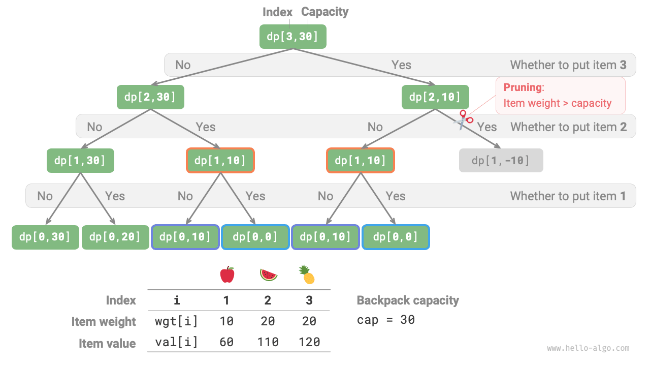
As shown in Figure 14-18, since each item generates two search branches of not selecting and selecting, the time complexity is \(O(2^n)\).
Observing the recursive tree, it is easy to see that there are overlapping sub-problems, such as \(dp[1, 10]\), etc. When there are many items and the knapsack capacity is large, especially when there are many items of the same weight, the number of overlapping sub-problems will increase significantly.
Figure 14-18 The brute force search recursive tree of the 0-1 knapsack problem
2. Method two: Memoized search
To ensure that overlapping sub-problems are only calculated once, we use a memoization list mem to record the solutions to sub-problems, where mem[i][c] corresponds to \(dp[i, c]\).
After introducing memoization, the time complexity depends on the number of sub-problems, which is \(O(n \times cap)\). The implementation code is as follows:
def knapsack_dfs_mem(
    wgt: list[int], val: list[int], mem: list[list[int]], i: int, c: int
) -> int:
    """0-1 Knapsack: Memoized search"""
    # If all items have been chosen or the knapsack has no remaining capacity, return value 0
    if i == 0 or c == 0:
        return 0
    # If there is a record, return it
    if mem[i][c] != -1:
        return mem[i][c]
    # If exceeding the knapsack capacity, can only choose not to put it in the knapsack
    if wgt[i - 1] > c:
        return knapsack_dfs_mem(wgt, val, mem, i - 1, c)
    # Calculate the maximum value of not putting in and putting in item i
    no = knapsack_dfs_mem(wgt, val, mem, i - 1, c)
    yes = knapsack_dfs_mem(wgt, val, mem, i - 1, c - wgt[i - 1]) + val[i - 1]
    # Record and return the greater value of the two options
    mem[i][c] = max(no, yes)
    return mem[i][c]
/* 0-1 Knapsack: Memoized search */
int knapsackDFSMem(int[] wgt, int[] val, int[][] mem, int i, int c) {
    // If all items have been chosen or the knapsack has no remaining capacity, return value 0
    if (i == 0 || c == 0) {
        return 0;
    }
    // If there is a record, return it
    if (mem[i][c] != -1) {
        return mem[i][c];
    }
    // If exceeding the knapsack capacity, can only choose not to put it in the knapsack
    if (wgt[i - 1] > c) {
        return knapsackDFSMem(wgt, val, mem, i - 1, c);
    }
    // Calculate the maximum value of not putting in and putting in item i
    int no = knapsackDFSMem(wgt, val, mem, i - 1, c);
    int yes = knapsackDFSMem(wgt, val, mem, i - 1, c - wgt[i - 1]) + val[i - 1];
    // Record and return the greater value of the two options
    mem[i][c] = Math.max(no, yes);
    return mem[i][c];
}
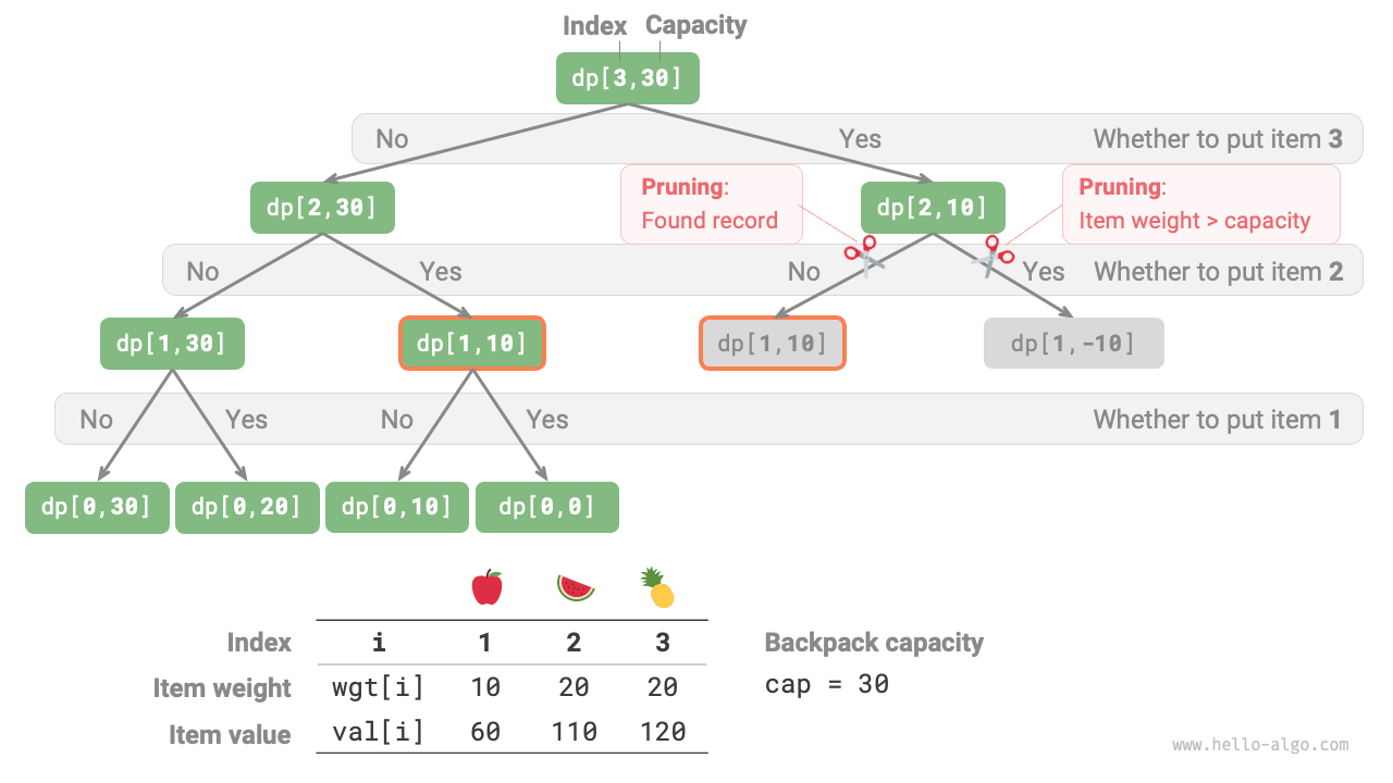
Figure 14-19 shows the search branches that are pruned in memoized search.
Figure 14-19 The memoized search recursive tree of the 0-1 knapsack problem
3. Method three: Dynamic programming
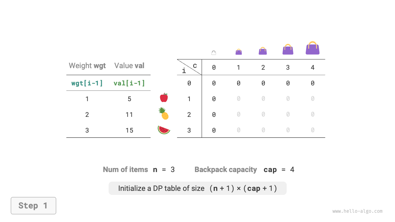
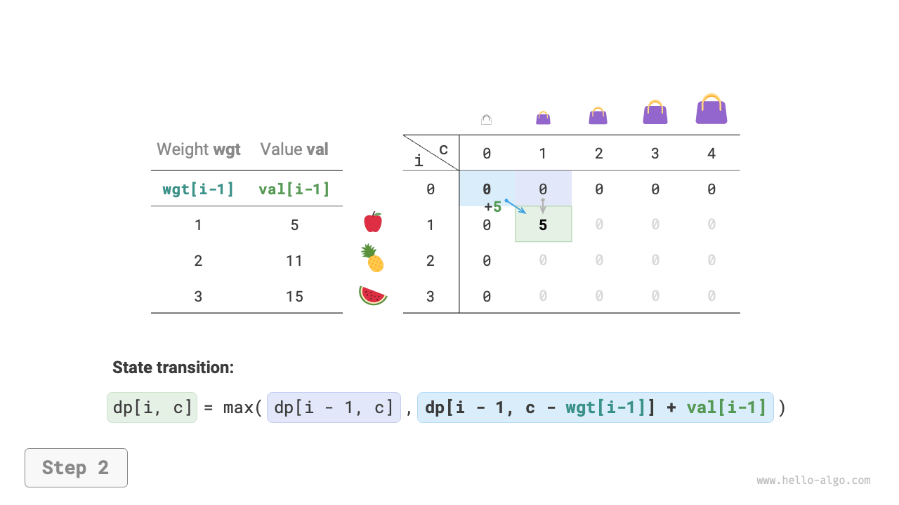
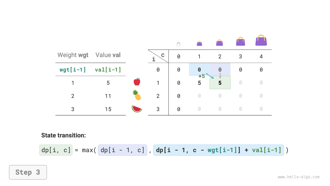
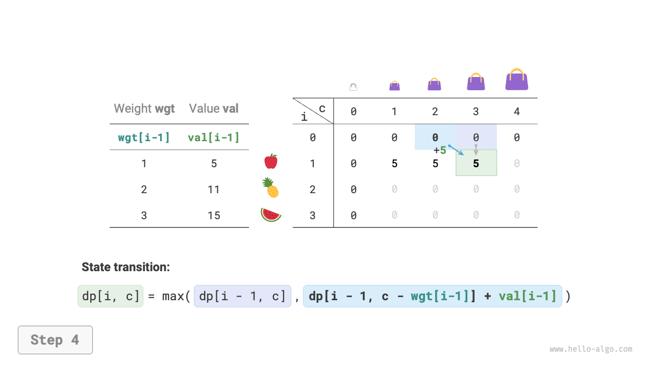
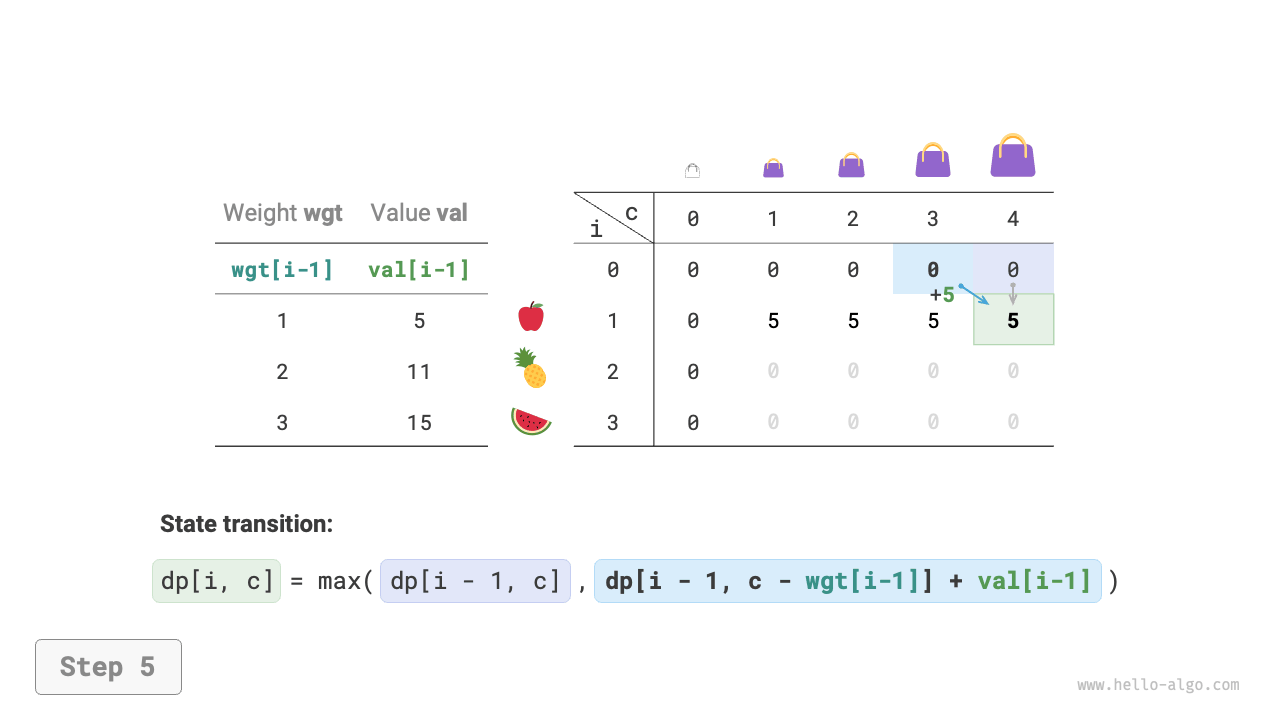
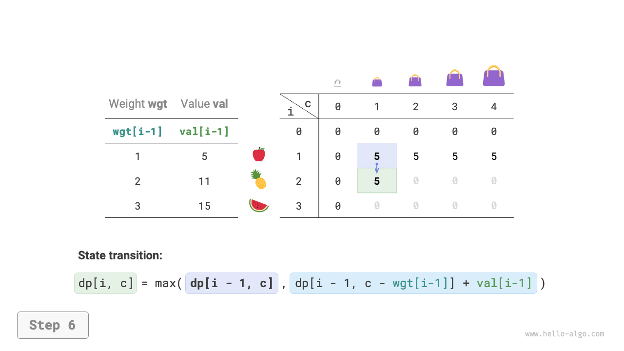
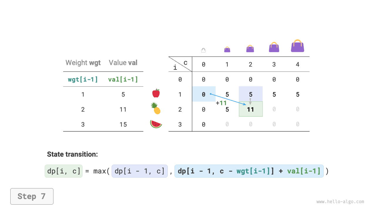
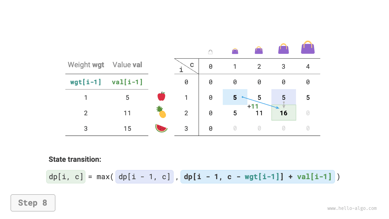
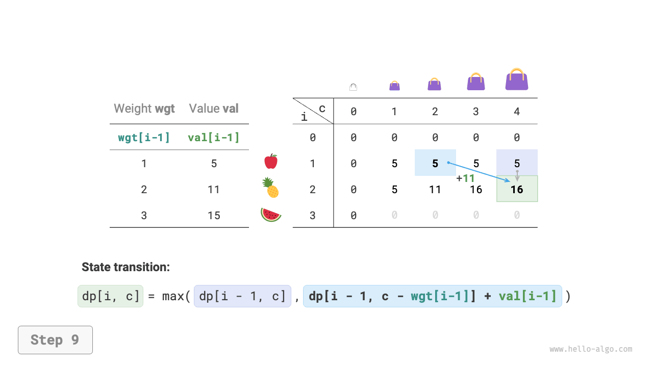
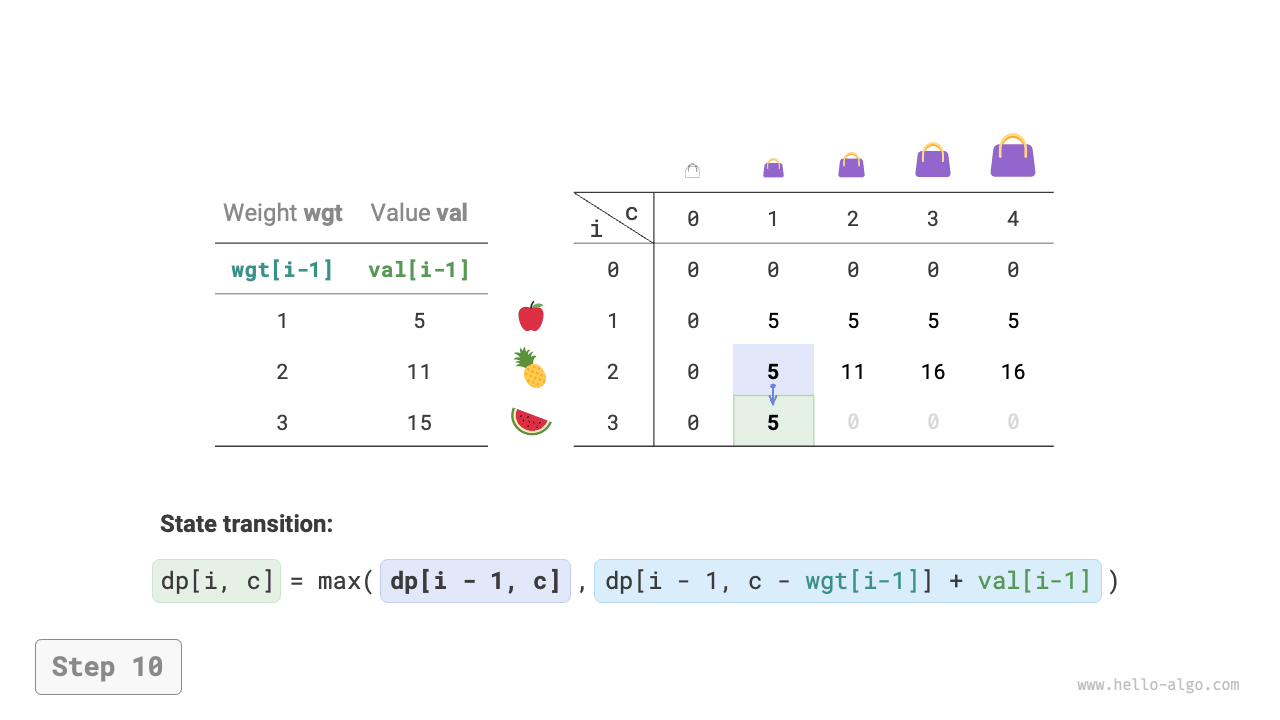
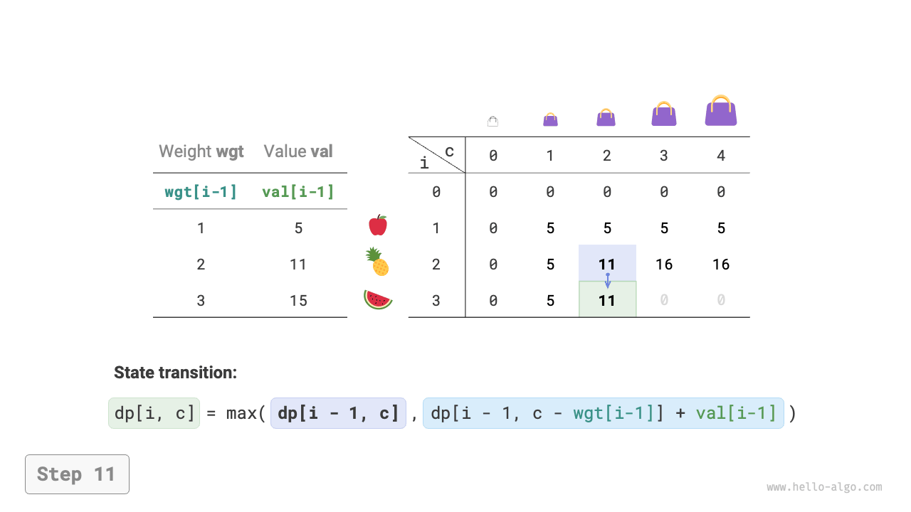
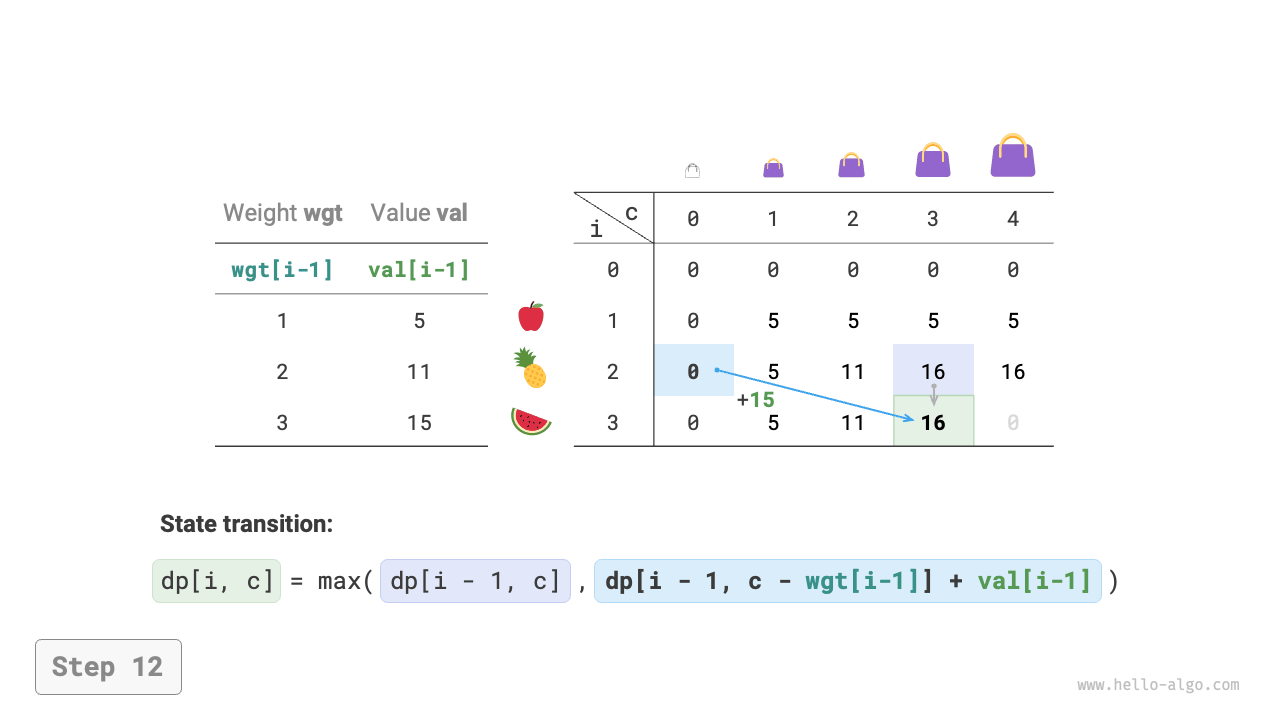
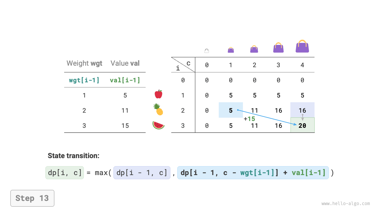
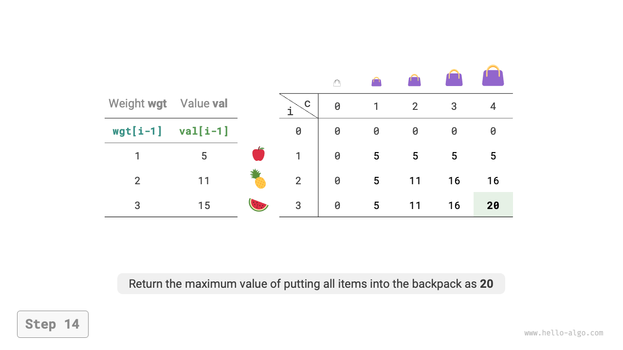
Dynamic programming essentially involves filling the \(dp\) table during the state transition, the code is shown in Figure 14-20:
def knapsack_dp(wgt: list[int], val: list[int], cap: int) -> int:
    """0-1 Knapsack: Dynamic programming"""
    n = len(wgt)
    # Initialize dp table
    dp = [[0] * (cap + 1) for _ in range(n + 1)]
    # State transition
    for i in range(1, n + 1):
        for c in range(1, cap + 1):
            if wgt[i - 1] > c:
                # If exceeding the knapsack capacity, do not choose item i
                dp[i][c] = dp[i - 1][c]
            else:
                # The greater value between not choosing and choosing item i
                dp[i][c] = max(dp[i - 1][c], dp[i - 1][c - wgt[i - 1]] + val[i - 1])
    return dp[n][cap]
/* 0-1 Knapsack: Dynamic programming */
int knapsackDP(int[] wgt, int[] val, int cap) {
    int n = wgt.length;
    // Initialize dp table
    int[][] dp = new int[n + 1][cap + 1];
    // State transition
    for (int i = 1; i <= n; i++) {
        for (int c = 1; c <= cap; c++) {
            if (wgt[i - 1] > c) {
                // If exceeding the knapsack capacity, do not choose item i
                dp[i][c] = dp[i - 1][c];
            } else {
                // The greater value between not choosing and choosing item i
                dp[i][c] = Math.max(dp[i - 1][c], dp[i - 1][c - wgt[i - 1]] + val[i - 1]);
            }
        }
    }
    return dp[n][cap];
}
As shown in the figures below, both the time complexity and space complexity are determined by the size of the array dp, i.e., \(O(n \times cap)\).
Figure 14-20 The dynamic programming process of the 0-1 knapsack problem
4. Space optimization
Since each state is only related to the state in the row above it, we can use two arrays to roll forward, reducing the space complexity from \(O(n^2)\) to \(O(n)\).
Further thinking, can we use just one array to achieve space optimization? It can be observed that each state is transferred from the cell directly above or from the upper left cell. If there is only one array, when starting to traverse the \(i\)-th row, that array still stores the state of row \(i-1\).
- If using normal order traversal, then when traversing to \(dp[i, j]\), the values from the upper left \(dp[i-1, 1]\) ~ \(dp[i-1, j-1]\) may have already been overwritten, thus the correct state transition result cannot be obtained.
- If using reverse order traversal, there will be no overwriting problem, and the state transition can be conducted correctly.
The figures below show the transition process from row \(i = 1\) to row \(i = 2\) in a single array. Please think about the differences between normal order traversal and reverse order traversal.
Figure 14-21 The space-optimized dynamic programming process of the 0-1 knapsack
In the code implementation, we only need to delete the first dimension \(i\) of the array dp and change the inner loop to reverse traversal:
def knapsack_dp_comp(wgt: list[int], val: list[int], cap: int) -> int:
    """0-1 Knapsack: Space-optimized dynamic programming"""
    n = len(wgt)
    # Initialize dp table
    dp = [0] * (cap + 1)
    # State transition
    for i in range(1, n + 1):
        # Traverse in reverse order
        for c in range(cap, 0, -1):
            if wgt[i - 1] > c:
                # If exceeding the knapsack capacity, do not choose item i
                dp[c] = dp[c]
            else:
                # The greater value between not choosing and choosing item i
                dp[c] = max(dp[c], dp[c - wgt[i - 1]] + val[i - 1])
    return dp[cap]
/* 0-1 Knapsack: Space-optimized dynamic programming */
int knapsackDPComp(int[] wgt, int[] val, int cap) {
    int n = wgt.length;
    // Initialize dp table
    int[] dp = new int[cap + 1];
    // State transition
    for (int i = 1; i <= n; i++) {
        // Traverse in reverse order
        for (int c = cap; c >= 1; c--) {
            if (wgt[i - 1] <= c) {
                // The greater value between not choosing and choosing item i
                dp[c] = Math.max(dp[c], dp[c - wgt[i - 1]] + val[i - 1]);
            }
        }
    }
    return dp[cap];
}
